!pip install wget

Linear Regression

import copy
import pandas as pd
import numpy as np
import matplotlib as mpl
import matplotlib.pyplot as plt
import matplotlib.animation as animation
import seaborn as sns

cmap = plt.get_cmap("tab10")
colors = [cmap(i) for i in range(cmap.N)]

mpl.rcParams["font.size"] = 24
mpl.rcParams["lines.linewidth"] = 2

Load Dataset and Prepare Data

!python -m wget https://raw.githubusercontent.com/deepchem/deepchem/master/datasets/delaney-processed.csv \
    --output delaney-processed.csv

Saved under delaney-processed.csv

DELANEY_FILE = "delaney-processed.csv"
df = pd.read_csv(DELANEY_FILE)
print(f"Number of molecules in the dataset: {df.shape[0]}")

Number of molecules in the dataset: 1128

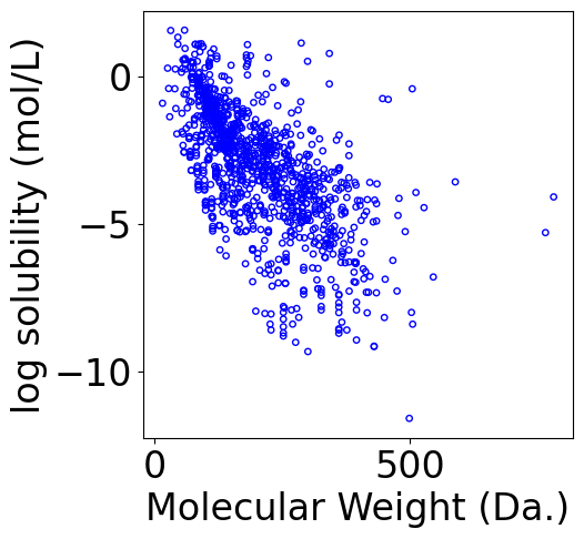
logS vs. Molecular Weight

# features
X = df[["Molecular Weight"]].values
X = X.reshape(-1, 1)
X = np.hstack([np.ones_like(X), X])

# ground truth
Y = df["measured log solubility in mols per litre"].values
Y = Y.reshape(-1, 1)

print("Shape of X:", X.shape)
print("Shape of Y:", Y.shape)

Shape of X: (1128, 2)
Shape of Y: (1128, 1)

f, ax = plt.subplots(1, 1, figsize=(5,5))
# scatter

ax.scatter(X[:, -1], Y.reshape(-1), \
            s=15, marker='o', \
            facecolors='none', edgecolor="blue")

ax.set_xlabel("Molecular Weight (Da.)")
ax.set_ylabel("log solubility (mol/L)")

Text(0, 0.5, 'log solubility (mol/L)')

Analytical solution

theta = np.linalg.inv((X.T @ X)) @ (X.T @ Y)

theta

array([[-0.38596872],
       [-0.01306351]])

Loss

y_pred = X @ theta
loss = np.mean((y_pred - Y)**2)
print(f"Loss: {loss}")

Loss: 2.5914815319019286

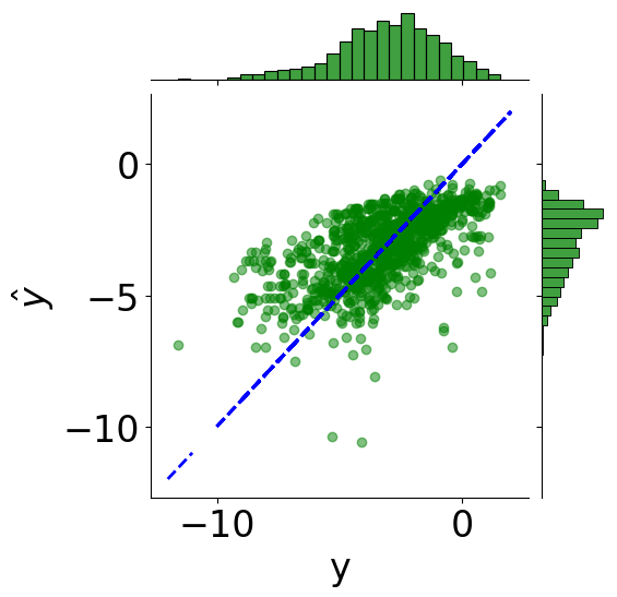
Plot Correlation

min_logS = np.min(Y)
max_logS = np.max(Y)
x_line = np.linspace(np.floor(min_logS), np.ceil(max_logS), 100)

tmp_df = pd.DataFrame({"y": Y.reshape(-1), r"$\hat{y}$": y_pred.reshape(-1)})

# scatter plot
g = sns.JointGrid(x="y", y=r"$\hat{y}$", data=tmp_df)
g = g.plot_joint(plt.scatter, c="green", alpha=0.5)

# line: y_pred = y
y_line = np.linspace(np.floor(Y.reshape(-1)), np.ceil(Y.reshape(-1)), 200)
g.ax_joint.plot(y_line, y_line, color="blue", linestyle="--");

# histograms
g = g.plot_marginals(sns.histplot, data=df, color="green", kde=False)

from sklearn.metrics import r2_score
print(f"Coefficient of determination: {r2_score(Y.reshape(-1), y_pred):.2f}")

Coefficient of determination: 0.41

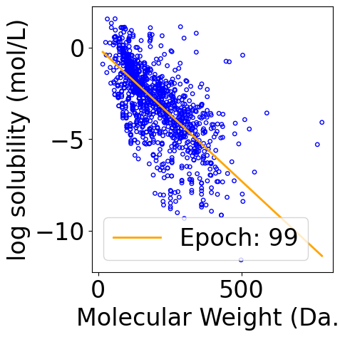
Plot the regression line

f, ax = plt.subplots(1, 1, figsize=(5,5))

plt.tight_layout()
ax.scatter(X[:, -1], Y.reshape(-1), \
            s=15, marker='o', \
            facecolors='none', edgecolor="blue")

min_X = np.min(X[:, -1])
max_X = np.max(X[:, -1])
x_line = np.linspace(np.floor(min_X), np.ceil(max_X), 100)
x_line = x_line.reshape(-1, 1)
x_line = np.hstack([np.ones_like(x_line), x_line])
y_pred_line = x_line @ theta

line, = ax.plot(x_line[:, -1], y_pred_line, color="orange", label="Fitted line")

ax.set_xlabel("Molecular Weight (Da.)")
ax.set_ylabel("log solubility (mol/L)")

Text(-6.152777777777777, 0.5, 'log solubility (mol/L)')

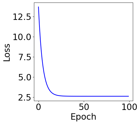
Gradient Descent

lr = 1e-6

theta_list = []
loss_list = []
# theta = np.random.randn(2, 1).reshape(-1, 1)
theta = np.array([0, 0]).reshape(-1, 1)
n_epochs = 100

for _ in range(n_epochs):
    theta_list.append(copy.deepcopy(theta))
    y_pred = X @ theta
    loss = np.mean((y_pred - Y).reshape(-1)**2)
    loss_list.append(loss)
    grad = 2*X.T @ (X @ theta - Y) / Y.shape[0]
    theta = theta - lr * grad

print("Final loss:", loss_list[-1])

Final loss: 2.6216033000052184

f, ax = plt.subplots(1, 1, figsize=(5,5))

ax.plot(loss_list, c="blue")
plt.xlabel("Epoch")
plt.ylabel("Loss")

Text(0, 0.5, 'Loss')

Plot Iterative Process

f, ax = plt.subplots(1, 1, figsize=(5, 5))

plt.tight_layout()
ax.scatter(X[:, -1], Y.reshape(-1), \
            s=15, marker='o', \
            facecolors='none', edgecolor="blue")

min_X = np.min(X[:, -1])
max_X = np.max(X[:, -1])
x_line = np.linspace(np.floor(min_X), np.ceil(max_X), 100)
x_line = x_line.reshape(-1, 1)
x_line = np.hstack([np.ones_like(x_line), x_line])

line, = ax.plot([], [], color="orange", label="")

ax.set_xlabel("Molecular Weight (Da.)")
ax.set_ylabel("log solubility (mol/L)")

legend = plt.legend(loc="upper right")

def animate(i):
    y_pred_line = x_line @ theta_list[i]
    line.set_data(x_line[:, -1], y_pred_line)
    line.set_label(f"Epoch: {i}")
    legend = plt.legend()
    return line, legend


ani = animation.FuncAnimation(f, animate, repeat=True, frames=len(theta_list), interval=100, blit=True)

writer = animation.PillowWriter(fps=10,
                                metadata=dict(artist='Me'),
                                bitrate=1800)
ani.save("theta_iteration.gif", writer=writer)

/tmp/ipython-input-4040914613.py:19: UserWarning: No artists with labels found to put in legend.  Note that artists whose label start with an underscore are ignored when legend() is called with no argument.
  legend = plt.legend(loc="upper right")

Data Normalization in Gradient Descent

from sklearn.preprocessing import StandardScaler

scaler = StandardScaler()
norm_mw = scaler.fit_transform(df[["Molecular Weight"]].values)
X = np.hstack([np.ones_like(norm_mw), norm_mw])

lr = 1e-1

theta_list = []
loss_list = []
# theta = np.random.randn(2, 1).reshape(-1, 1)
theta = np.array([0, 0]).reshape(-1, 1)
n_epochs = 20

for _ in range(n_epochs):
    theta_list.append(copy.deepcopy(theta))
    y_pred = X @ theta
    loss = np.mean((y_pred - Y).reshape(-1)**2)
    loss_list.append(loss)
    grad = 2*X.T @ (X @ theta - Y) / Y.shape[0]
    theta = theta - lr * grad

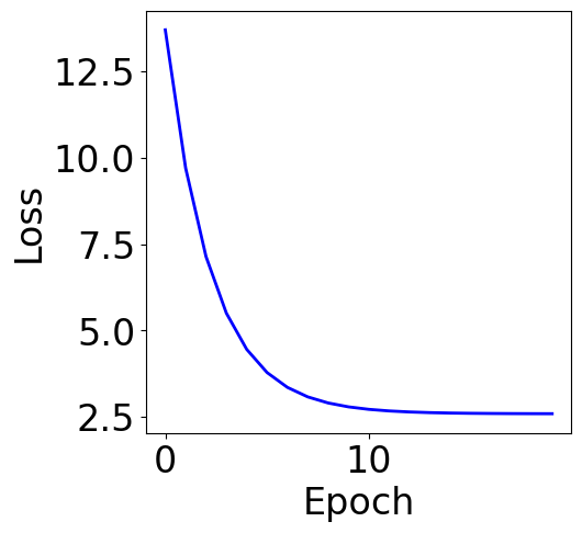
print("Final loss:", loss_list[-1])

Final loss: 2.593787495277282

Plot Training Curve

f, ax = plt.subplots(1, 1, figsize=(5,5))

ax.plot(loss_list, c="blue")
plt.xlabel("Epoch")
plt.ylabel("Loss")

Text(0, 0.5, 'Loss')

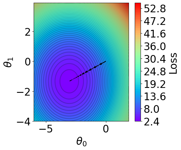
Parameter Contour

def V(xx, yy):
    losses = []
    theta = np.hstack([xx.reshape(-1, 1), yy.reshape(-1, 1)])
    for i in range(theta.shape[0]):
        y_pred = X @ theta[i].reshape(-1, 1)
        loss = np.mean((y_pred - Y).reshape(-1)**2)
        losses.append(loss)
    return np.array(losses)

# calculate contour
t1 = np.arange(-6, 2, 1e-1)
t2 = np.arange(-4, 4, 1e-1)
xx, yy = np.meshgrid(t1, t2)
z = V(xx.ravel(), yy.ravel()).reshape(len(t2), -1)

fig,ax = plt.subplots(1,1,figsize=(5,5))

n_levels = 75
c = ax.contourf(t1, t2, z, cmap='rainbow', levels=n_levels, zorder=1)
ax.contour(t1,t2, z, levels=n_levels, zorder=1, colors='black', alpha=0.2)
cb = fig.colorbar(c)
cb.set_label("Loss")

r=0.1
g=0.1
b=0.2
ax.patch.set_facecolor((r,g,b,.15))


# plot trajectory
for i in range(len(theta_list)-1):
    plt.quiver(theta_list[i][0], theta_list[i][1], # from point
               theta_list[i+1][0]-theta_list[i][0],  theta_list[i+1][1]-theta_list[i][1], # to point:
               angles="xy", scale_units="xy", scale=1, color="black",
               linewidth=1.5)


ax.set_xlabel(r'$\theta_0$')
ax.set_ylabel(r'$\theta_1$')

Text(0, 0.5, '$\\theta_1$')

Stochastic Gradient Descent and Mini-batching

lr = 1e-1

theta_list = []
loss_list = []
theta = np.array([0, 0]).reshape(-1, 1)
n_epochs = 100
batch_size = 32 # change the batch size here

for _ in range(n_epochs):
    indices = np.random.choice(X.shape[0], batch_size, replace=False)
    theta_list.append(copy.deepcopy(theta))
    y_pred = X[indices, :] @ theta
    y_true = Y[indices]
    loss = np.mean((y_pred - y_true).reshape(-1)**2)
    loss_list.append(loss)
    grad = 2*X[indices, :].T @ (y_pred - y_true) / len(indices)
    theta = theta - lr * grad

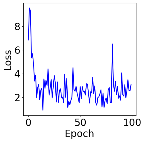
print("Final loss:", pd.Series(loss_list).rolling(5).mean().iloc[-1])

Final loss: 2.8454754567289027

Plot Training CUrve

f, ax = plt.subplots(1, 1, figsize=(5,5))

ax.plot(loss_list, c="blue")
plt.xlabel("Epoch")
plt.ylabel("Loss")

Text(0, 0.5, 'Loss')

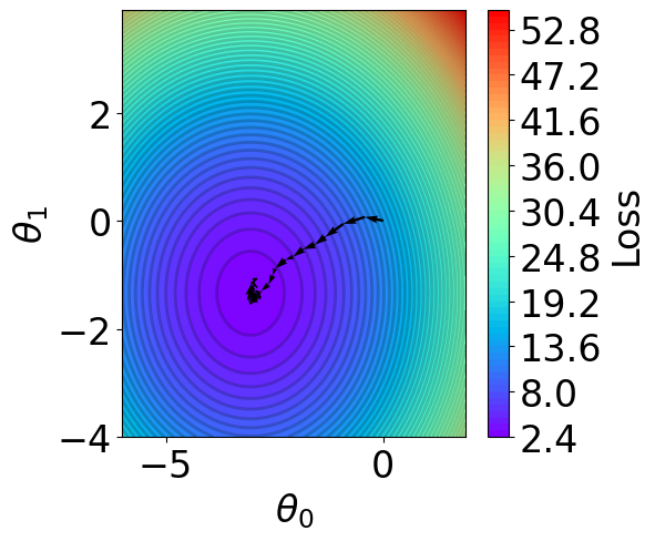
Parameter Contour

def V(xx, yy):
    losses = []
    theta = np.hstack([xx.reshape(-1, 1), yy.reshape(-1, 1)])
    for i in range(theta.shape[0]):
        y_pred = X @ theta[i].reshape(-1, 1)
        loss = np.mean((y_pred - Y).reshape(-1)**2)
        losses.append(loss)
    return np.array(losses)

# calculate contour
region = np.stack(theta_list)

t1 = np.arange(-6, 2, 1e-1)
t2 = np.arange(-4, 4, 1e-1)
xx, yy = np.meshgrid(t1, t2)
z = V(xx.ravel(), yy.ravel()).reshape(len(t2), -1)

fig,ax = plt.subplots(1,1,figsize=(5,5))

# z = np.ma.masked_greater(z, 10)
n_levels = 75
c = ax.contourf(t1, t2, z, cmap='rainbow', levels=n_levels, zorder=1)
ax.contour(t1,t2, z, levels=n_levels, zorder=1, colors='black', alpha=0.2)
cb = fig.colorbar(c)
cb.set_label("Loss")

r=0.1
g=0.1
b=0.2
ax.patch.set_facecolor((r,g,b,.15))


# plot trajectory

for i in range(50):
    plt.quiver(theta_list[i][0], theta_list[i][1], # from point
               theta_list[i+1][0]-theta_list[i][0],  theta_list[i+1][1]-theta_list[i][1], # to point:
               angles="xy", scale_units="xy", scale=1, color="black",
               linewidth=1.5)


ax.set_xlabel(r'$\theta_0$')
ax.set_ylabel(r'$\theta_1$')

Text(0, 0.5, '$\\theta_1$')