!pip install wget

Avoid Overfitting using Regularization

import copy
import random
import numpy as np
import pandas as pd
import matplotlib.pyplot as plt
import matplotlib as mpl
import seaborn as sns
mpl.rcParams["font.size"] = 20
mpl.rcParams["lines.linewidth"] = 2

from sklearn.preprocessing import PolynomialFeatures
from sklearn.linear_model import LinearRegression
from sklearn.decomposition import PCA
from sklearn.manifold import TSNE
from sklearn.preprocessing import StandardScaler
from sklearn.model_selection import train_test_split
from sklearn.model_selection import KFold


def seed_all(seed):
    random.seed(seed)
    np.random.seed(seed)

# for the purpose of reproduce
SEED = 0
seed_all(SEED)

Load Dataset

!python -m wget https://raw.githubusercontent.com/deepchem/deepchem/master/datasets/delaney-processed.csv \
    --output delaney-processed.csv

DELANEY_FILE = "delaney-processed.csv"
TASK_COL = 'measured log solubility in mols per litre'
df = pd.read_csv(DELANEY_FILE)
print(f"Number of molecules in the dataset: {df.shape[0]}")

Number of molecules in the dataset: 1128

df

	Compound ID	ESOL predicted log solubility in mols per litre	Minimum Degree	Molecular Weight	Number of H-Bond Donors	Number of Rings	Number of Rotatable Bonds	Polar Surface Area	measured log solubility in mols per litre	smiles
0	Amigdalin	-0.974	1	457.432	7	3	7	202.32	-0.770	OCC3OC(OCC2OC(OC(C#N)c1ccccc1)C(O)C(O)C2O)C(O)...
1	Fenfuram	-2.885	1	201.225	1	2	2	42.24	-3.300	Cc1occc1C(=O)Nc2ccccc2
2	citral	-2.579	1	152.237	0	0	4	17.07	-2.060	CC(C)=CCCC(C)=CC(=O)
3	Picene	-6.618	2	278.354	0	5	0	0.00	-7.870	c1ccc2c(c1)ccc3c2ccc4c5ccccc5ccc43
4	Thiophene	-2.232	2	84.143	0	1	0	0.00	-1.330	c1ccsc1
...	...	...	...	...	...	...	...	...	...	...
1123	halothane	-2.608	1	197.381	0	0	0	0.00	-1.710	FC(F)(F)C(Cl)Br
1124	Oxamyl	-0.908	1	219.266	1	0	1	71.00	0.106	CNC(=O)ON=C(SC)C(=O)N(C)C
1125	Thiometon	-3.323	1	246.359	0	0	7	18.46	-3.091	CCSCCSP(=S)(OC)OC
1126	2-Methylbutane	-2.245	1	72.151	0	0	1	0.00	-3.180	CCC(C)C
1127	Stirofos	-4.320	1	365.964	0	1	5	44.76	-4.522	COP(=O)(OC)OC(=CCl)c1cc(Cl)c(Cl)cc1Cl

1128 rows × 10 columns

Polynomial Fitting

X = df[["Molecular Weight", "Number of H-Bond Donors", "Number of Rings", "Number of Rotatable Bonds"]].values
y = df[TASK_COL].values.reshape(-1, 1)

test_size = int(len(X)*0.1)
X_train, X_test, y_train, y_test = train_test_split(X, y, test_size=test_size, shuffle=True)

def run_gd(X_train, y_train, X_test, y_test, lr, M,
           n_epochs=20, normalize=True, norm=None,
           lamda=1, init="zero", return_mse=True):
    assert init in ["zero", "random"]
    theta_list = []
    loss_list = []
    loss_test_list = []
    if return_mse:
        mse_list = []
        mse_test_list = []

    poly_features = PolynomialFeatures(degree=M)
    X_train_poly = poly_features.fit_transform(X_train)
    X_test_poly = poly_features.fit_transform(X_test)

    if normalize:
        scaler = StandardScaler()
        X_train_poly = scaler.fit_transform(X_train_poly)
        X_test_poly = scaler.transform(X_test_poly)
    else:
        scaler = None

    X_train_poly = np.hstack([np.ones((X_train_poly.shape[0], 1)), X_train_poly])
    X_test_poly = np.hstack([np.ones((X_test_poly.shape[0], 1)), X_test_poly])

    if init == "zero":
        theta = np.zeros(X_train_poly.shape[1]).reshape(-1, 1)
    else:
        theta = np.random.randn(X_train_poly.shape[1]).reshape(-1, 1)

    # gd fit
    for _ in range(n_epochs):
        theta_list.append(copy.deepcopy(theta))

        y_pred = X_train_poly @ theta
        loss = np.mean((y_pred - y_train).reshape(-1)**2)
        if return_mse:
            mse_list.append(loss)
        if norm is None:
            loss = loss
        elif norm == "l1":
            loss += lamda*np.sum(np.abs(theta))
        elif norm == "l2":
            loss += lamda*np.sum(theta**2)
        else:
            NotImplementedError(f"Norm {norm} is not valid normalization method")
        loss_list.append(loss)
        grad = 2*X_train_poly.T @ (X_train_poly @ theta - y_train) / y_train.shape[0]
        if norm is None:
            grad = grad
        elif norm == "l1":
            grad += lamda*np.sign(theta)
        elif norm == "l2":
            grad += lamda*2*theta
        else:
            raise NotImplementedError(f"Norm {norm} is not valid normalization method")

        theta = theta - lr * grad

        # predict and calculate rmse of test dataset
        y_test_pred = X_test_poly @ theta
        loss_test = np.mean((y_test_pred-y_test).reshape(-1)**2)
        if return_mse:
            mse_test_list.append(loss_test)
        if norm is None:
            loss_test = loss_test
        elif norm == "l1":
            loss_test += lamda*np.sum(np.abs(theta))
        elif norm == "l2":
            loss_test += lamda*np.sum(theta**2)
        else:
            NotImplementedError(f"Norm {norm} is not valid normalization method")
        loss_test_list.append(loss_test)
    if return_mse:
        return theta_list, mse_list, mse_test_list, scaler
    else:
        return theta_list, loss_list, loss_test_list, scaler

Without Regularization

lr = 5e-3
n_epochs = 1500
normalize = True
norm = None # regularization in GD

orders = [0, 1, 2, 3, 4, 5]
results = {}

for idx, M in enumerate(orders):
    theta_list, loss_list, loss_test_list, scaler = run_gd(X_train, y_train, X_test, y_test, lr, M, n_epochs, normalize)
    results[M] = (theta_list, loss_list, loss_test_list, scaler)

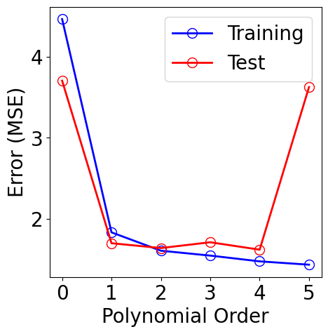
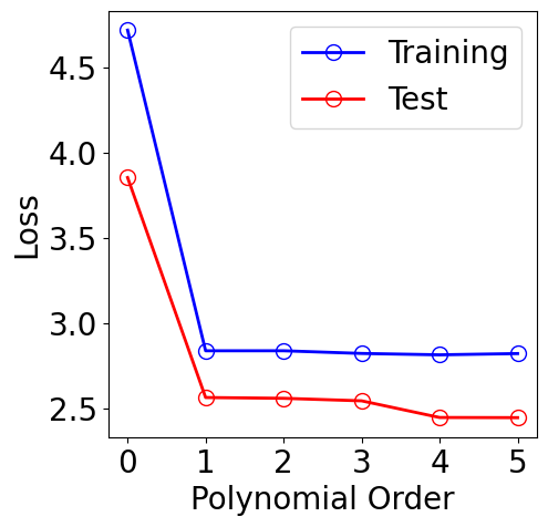
plt.figure(figsize=(5, 5))
plt.plot(orders, [results[M][1][-1] for M in orders], "-", color="b",
         marker="o", markersize=10, markerfacecolor="none", markeredgecolor="b", label="Training")
plt.plot(orders, [results[M][2][-1] for M in orders], "-", color="r",
         marker="o", markersize=10, markerfacecolor="none", markeredgecolor="r", label="Test")
plt.xlabel("Polynomial Order")
plt.ylabel("Error (MSE)")
plt.xticks(orders)
plt.legend()

<matplotlib.legend.Legend at 0x7ac9f2eac0d0>

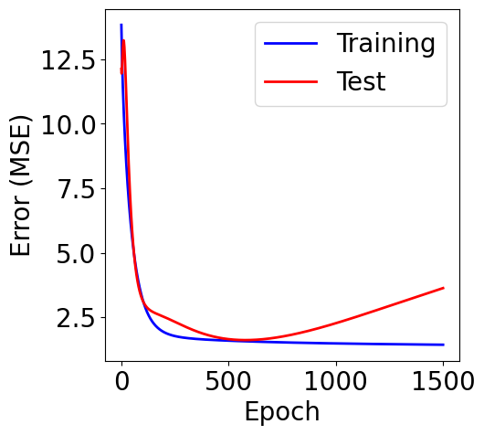
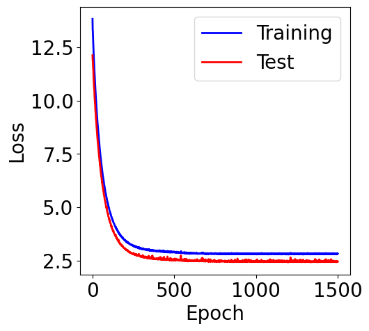
M = orders[-1]
theta_list, loss_list, loss_test_list, scaler = results[M]

f, ax = plt.subplots(1, 1, figsize=(5,5))

ax.plot(loss_list, c="blue", label="Training")
ax.plot(loss_test_list, c="red", label="Test")
plt.xlabel("Epoch")
plt.ylabel("Error (MSE)")
plt.legend()

<matplotlib.legend.Legend at 0x7ac9f06a5090>

L2 Norm

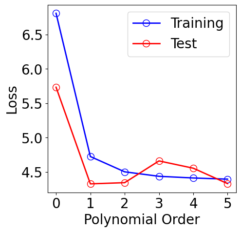
normalize = True
norm = "l2" # regularization in GD
lamda = 1

results = {}


for idx, M in enumerate(orders):
    theta_list, loss_list, loss_test_list, scaler = run_gd(X_train, y_train, X_test, y_test,
                                                           lr, M, n_epochs, normalize, norm=norm, lamda=lamda)
    results[M] = (theta_list, loss_list, loss_test_list, scaler)

plt.figure(figsize=(5, 5))
plt.plot(orders, [results[M][1][-1] for M in orders], "-", color="b",
         marker="o", markersize=10, markerfacecolor="none", markeredgecolor="b", label="Training")
plt.plot(orders, [results[M][2][-1] for M in orders], "-", color="r",
         marker="o", markersize=10, markerfacecolor="none", markeredgecolor="r", label="Test")
plt.xlabel("Polynomial Order")
plt.ylabel("Loss")
plt.xticks(orders)
plt.legend()

<matplotlib.legend.Legend at 0x7ac9f0692210>

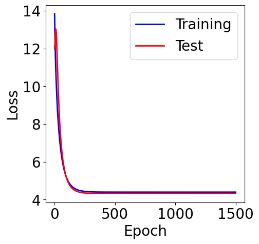
M = orders[-1]
theta_list, loss_list, loss_test_list, scaler = results[M]

f, ax = plt.subplots(1, 1, figsize=(5,5))

ax.plot(loss_list, c="blue", label="Training")
ax.plot(loss_test_list, c="red", label="Test")
plt.xlabel("Epoch")
plt.ylabel("Loss")
plt.legend()

<matplotlib.legend.Legend at 0x7aca2a3b3710>

L1 Norm

normalize = True
norm = "l1" # regularization in GD
lamda = 1

results = {}

for idx, M in enumerate(orders):
    theta_list, loss_list, loss_test_list, scaler = run_gd(X_train, y_train, X_test, y_test,
                                                           lr, M, n_epochs, normalize, norm=norm, lamda=lamda)
    results[M] = (theta_list, loss_list, loss_test_list, scaler)

plt.figure(figsize=(5, 5))
plt.plot(orders, [results[M][1][-1] for M in orders], "-", color="b",
         marker="o", markersize=10, markerfacecolor="none", markeredgecolor="b", label="Training")
plt.plot(orders, [results[M][2][-1] for M in orders], "-", color="r",
         marker="o", markersize=10, markerfacecolor="none", markeredgecolor="r", label="Test")
plt.xlabel("Polynomial Order")
plt.ylabel("Loss")
plt.xticks(orders)
plt.legend()

<matplotlib.legend.Legend at 0x7ac9f06a5850>

M = orders[-1]
theta_list, loss_list, loss_test_list, scaler = results[M]

f, ax = plt.subplots(1, 1, figsize=(5,5))

ax.plot(loss_list, c="blue", label="Training")
ax.plot(loss_test_list, c="red", label="Test")
plt.xlabel("Epoch")
plt.ylabel("Loss")
plt.legend()

<matplotlib.legend.Legend at 0x7ac9f0485b50>