[ ]:
!pip install wget
K-nearest Neighbour
[2]:
import pandas as pd
import numpy as np
from matplotlib import pyplot as plt


Download Datasets
[3]:
!python -m wget https://raw.githubusercontent.com/xuhuihuang/uwmadisonchem361/refs/heads/main/delaney_dataset_200compounds.csv \
--output delaney_dataset_200compounds.csv

!python -m wget https://raw.githubusercontent.com/xuhuihuang/uwmadisonchem361/refs/heads/main/delaney_dataset_40compounds.csv \
--output delaney_dataset_40compounds.csv

!python -m wget https://raw.githubusercontent.com/xuhuihuang/uwmadisonchem361/refs/heads/main/delaney_dataset_44compounds_with_outliers.csv \
--output delaney_dataset_44compounds_with_outliers.csv
Saved under delaney_dataset_200compounds.csv

Saved under delaney_dataset_40compounds.csv

Saved under delaney_dataset_44compounds_with_outliers.csv
Load the curated Delaney dataset, which contains 40 compounds:
20 Soluble Compounds: Defined as those with a “measured log solubility in mols per litre” ≥ -2, labeled as 1.
20 Non-Soluble Compounds: Defined as those with a “measured log solubility in mols per litre” < -2, labeled as -1.
[4]:
df = pd.read_csv('delaney_dataset_40compounds.csv')
df.head(2)
[4]:
| Molecular Weight | Polar Surface Area | measured log solubility in mols per litre | solubility labels | smiles | |
|---|---|---|---|---|---|
| 0 | 103.124 | 23.79 | -1.00 | 1 | N#Cc1ccccc1 |
| 1 | 116.204 | 20.23 | -1.81 | 1 | CCCCCCCO |
[5]:
data = df.iloc[:].values
[6]:
# data with log solubility and Polar Surface Are as features.
X = data[:,[2,1]]

# solubility labels
y = data[:,3].astype(int)
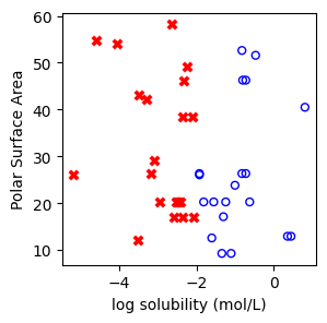
[7]:
f, ax = plt.subplots(1,1,figsize=(3,3))

ax.scatter(X[np.where(y==1)[0],0],X[np.where(y==1)[0],1],s=25, marker='o', facecolors='none', edgecolor="blue", label='soluble')
ax.scatter(X[np.where(y==-1)[0],0],X[np.where(y==-1)[0],1],s=50, marker='X', color='red',linewidths=0.1, label='non-soluble')

ax.set_xlabel("log solubility (mol/L)")
ax.set_ylabel("Polar Surface Area")
#plt.legend()
[7]:
Text(0, 0.5, 'Polar Surface Area')
Let’s fit a 1-NN model
[8]:
from sklearn.neighbors import KNeighborsClassifier

neigh = KNeighborsClassifier(n_neighbors=1)
neigh.fit(X, y)
[8]:
KNeighborsClassifier(n_neighbors=1)In a Jupyter environment, please rerun this cell to show the HTML representation or trust the notebook.
On GitHub, the HTML representation is unable to render, please try loading this page with nbviewer.org.
KNeighborsClassifier(n_neighbors=1)
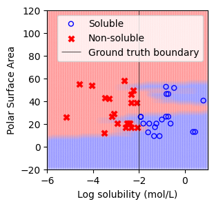
Visualize the predicted regions from 1-NN model.
In this visualization, the blue region indicates that the model predicts the points within this area as soluble and vice versa
As demonstrated, the performance of the 1-NN classifier is particularly sensitive to features that are either uncorrelated or unnormalized
[9]:
a = np.arange(-6,1.1,0.1)
b = np.arange(-20,121,1)
aa,bb = np.meshgrid(a,b)
X_grid = np.concatenate([aa.ravel().reshape(-1,1),bb.ravel().reshape(-1,1)],axis=1)
predict_labels = neigh.predict(X_grid)

from matplotlib.colors import ListedColormap

colors = ['red', 'blue']
cmap = ListedColormap(colors)

f, ax = plt.subplots(1,1,figsize=(3,3))
#plt.tight_layout(h_pad=0.5, w_pad=0.5, pad=2.5)
ax.scatter(x=X_grid[:,0], y=X_grid[:,1], c=predict_labels, cmap = cmap, alpha=0.025)

ax.scatter(X[np.where(y==1)[0],0],X[np.where(y==1)[0],1],s=25, marker='o', facecolors='none', edgecolor="blue", label='Soluble')
ax.scatter(X[np.where(y==-1)[0],0],X[np.where(y==-1)[0],1],s=50, marker='X', color='red',linewidths=0.1, label='Non-soluble')

ax.vlines(x=-2,ymin=-20,ymax=120,colors='black',linewidth=0.5,label='Ground truth boundary')

ax.set_xlabel("Log solubility (mol/L)")
ax.set_ylabel("Polar Surface Area")

ax.set_xlim(-6,1)
ax.set_ylim(-20,120)

plt.legend()
[9]:
<matplotlib.legend.Legend at 0x7e0c99563770>
[9]: