!pip install wget

Logistic regression

import pandas as pd
import numpy as np
from matplotlib import pyplot as plt

Download Datasets

!python -m wget https://raw.githubusercontent.com/xuhuihuang/uwmadisonchem361/refs/heads/main/delaney_dataset_200compounds.csv \
--output delaney_dataset_200compounds.csv

!python -m wget https://raw.githubusercontent.com/xuhuihuang/uwmadisonchem361/refs/heads/main/delaney_dataset_40compounds.csv \
--output delaney_dataset_40compounds.csv

!python -m wget https://raw.githubusercontent.com/xuhuihuang/uwmadisonchem361/refs/heads/main/delaney_dataset_44compounds_with_outliers.csv \
--output delaney_dataset_44compounds_with_outliers.csv

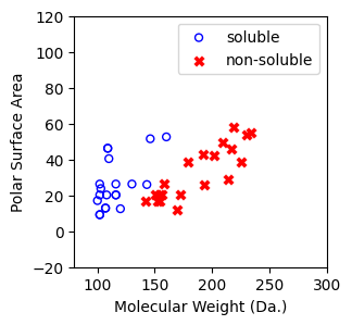
Load the curated Delaney dataset, which contains 40 compounds:

• 20 Soluble Compounds: Defined as those with a “measured log solubility in mols per litre” ≥ -2, labeled as 1.

• 20 Non-Soluble Compounds: Defined as those with a “measured log solubility in mols per litre” < -2, labeled as -1.

df = pd.read_csv('delaney_dataset_40compounds.csv')
df.head(2)

	Molecular Weight	Polar Surface Area	measured log solubility in mols per litre	solubility labels	smiles
0	103.124	23.79	-1.00	1	N#Cc1ccccc1
1	116.204	20.23	-1.81	1	CCCCCCCO

data = df.iloc[:].values

# data with Molecular Weight and Polar Surface Are as features.
X = data[:,0:2]

# solubility labels
y = data[:,3].astype(int)

visualize the 40 compounds

f, ax = plt.subplots(1,1,figsize=(3,3))

ax.scatter(X[np.where(y==1)[0],0],X[np.where(y==1)[0],1],s=25, marker='o', facecolors='none', edgecolor="blue", label='soluble')
ax.scatter(X[np.where(y==-1)[0],0],X[np.where(y==-1)[0],1],s=50, marker='X', color='red',linewidths=0.1, label='non-soluble')

ax.set_xlabel("Molecular Weight (Da.)")
ax.set_ylabel("Polar Surface Area")

ax.set_xlim(80,300)
ax.set_ylim(-20,120)

plt.legend()

<matplotlib.legend.Legend at 0x7cbbfe13aa80>

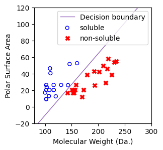
Fit a logistic regression model using sklearn

# plot the decision boundary
def predict_boundary(x,regressor):
    y = [(- regressor.coef_[0][0]*x[i] - regressor.intercept_)/(regressor.coef_[0][1]) for i in range(len(x))]
    return y

# coef_: Coefficient of the features in the decision function.
# coef_: Shape of (1, n_features) for binary classification - \theta_1 and \theta_2
# intercept_: \thetha_0
# Decision boundary line with x in the range of [80, 300].
# Decison line: p=0, so that y (polar surface) = [(-\theta_1*x (molecualr weight) - \theta_0)/\theta_1

from sklearn.linear_model import LogisticRegression

regressor = LogisticRegression(random_state=0,penalty=None).fit(X, y)

f, ax = plt.subplots(1,1,figsize=(3,3))

ax.plot(
    [80,300],
    predict_boundary([80,300],regressor=regressor),
    linewidth=1,
    color="tab:purple",
    label="Decision boundary",
)

ax.scatter(X[np.where(y==1)[0],0],X[np.where(y==1)[0],1],s=25, marker='o', facecolors='none', edgecolor="blue", label='soluble')
ax.scatter(X[np.where(y==-1)[0],0],X[np.where(y==-1)[0],1],s=50, marker='X', color='red',linewidths=0.1, label='non-soluble')

ax.set_xlabel("Molecular Weight (Da.)")
ax.set_ylabel("Polar Surface Area")

ax.set_xlim(80,300)
ax.set_ylim(-20,120)

plt.legend()

<matplotlib.legend.Legend at 0x7cbbf1574770>

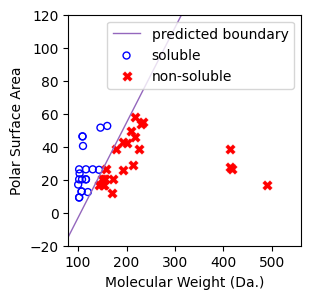
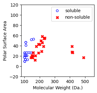
Logistic regression is robust to outliers

df = pd.read_csv('delaney_dataset_44compounds_with_outliers.csv')
df.head(2)

data = df.iloc[:].values

# data with Molecular Weight and Polar Surface Are as features.
X = data[:,0:2]

# solubility labels
y = data[:,3].astype(int)

f, ax = plt.subplots(1,1,figsize=(3,3))

ax.scatter(X[np.where(y==1)[0],0],X[np.where(y==1)[0],1],s=25, marker='o', facecolors='none', edgecolor="blue", label='soluble')
ax.scatter(X[np.where(y==-1)[0],0],X[np.where(y==-1)[0],1],s=50, marker='X', color='red',linewidths=0.1, label='non-soluble')

ax.set_xlabel("Molecular Weight (Da.)")
ax.set_ylabel("Polar Surface Area")

ax.set_xlim(80,560)
ax.set_ylim(-20,120)

plt.legend()

<matplotlib.legend.Legend at 0x7cbbf0ec40e0>

from sklearn.linear_model import LogisticRegression

regressor = LogisticRegression(random_state=0,penalty=None).fit(X, y)

f, ax = plt.subplots(1,1,figsize=(3,3))

ax.plot(
    [80,560],
    predict_boundary([80,560],regressor=regressor),
    linewidth=1,
    color="tab:purple",
    label="predicted boundary",
)

ax.scatter(X[np.where(y==1)[0],0],X[np.where(y==1)[0],1],s=25, marker='o', facecolors='none', edgecolor="blue", label='soluble')
ax.scatter(X[np.where(y==-1)[0],0],X[np.where(y==-1)[0],1],s=50, marker='X', color='red',linewidths=0.1, label='non-soluble')

ax.set_xlabel("Molecular Weight (Da.)")
ax.set_ylabel("Polar Surface Area")

ax.set_xlim(80,560)
ax.set_ylim(-20,120)

plt.legend()

<matplotlib.legend.Legend at 0x7cbbf1440c20>