[ ]:
!pip install wget
Decision Tree
[2]:
import pandas as pd
import numpy as np
from matplotlib import pyplot as plt
Download Datasets
[3]:
!python -m wget https://raw.githubusercontent.com/xuhuihuang/uwmadisonchem361/refs/heads/main/delaney_dataset_200compounds.csv \
--output delaney_dataset_200compounds.csv

!python -m wget https://raw.githubusercontent.com/xuhuihuang/uwmadisonchem361/refs/heads/main/delaney_dataset_40compounds.csv \
--output delaney_dataset_40compounds.csv

!python -m wget https://raw.githubusercontent.com/xuhuihuang/uwmadisonchem361/refs/heads/main/delaney_dataset_44compounds_with_outliers.csv \
--output delaney_dataset_44compounds_with_outliers.csv
Saved under delaney_dataset_200compounds.csv

Saved under delaney_dataset_40compounds.csv

Saved under delaney_dataset_44compounds_with_outliers.csv
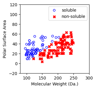
Load the curated Delaney dataset, which contains 200 compounds:
100 Soluble Compounds: Defined as those with a “measured log solubility in mols per litre” ≥ -2, labeled as 1.
100 Non-Soluble Compounds: Defined as those with a “measured log solubility in mols per litre” < -2, labeled as -1.
[4]:
df = pd.read_csv('delaney_dataset_200compounds.csv')
df.head(2)
[4]:
| Molecular Weight | Polar Surface Area | measured log solubility in mols per litre | solubility labels | smiles | |
|---|---|---|---|---|---|
| 0 | 103.124 | 23.79 | -1.00 | 1 | N#Cc1ccccc1 |
| 1 | 116.204 | 20.23 | -1.81 | 1 | CCCCCCCO |
[5]:
data = df.iloc[:].values
[6]:
# data with Molecular Weight and Polar Surface Are as features.
X = data[:,0:2]

# solubility labels
y = data[:,3].astype(int)
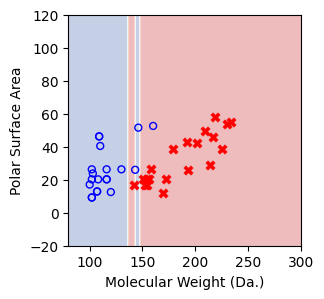
Visualize the 200 compounds
[7]:
f, ax = plt.subplots(1,1,figsize=(3,3))

ax.scatter(X[np.where(y==1)[0],0],X[np.where(y==1)[0],1],s=25, marker='o', facecolors='none', edgecolor="blue", label='soluble')
ax.scatter(X[np.where(y==-1)[0],0],X[np.where(y==-1)[0],1],s=50, marker='X', color='red',linewidths=0.1, label='non-soluble')

ax.set_xlabel("Molecular Weight (Da.)")
ax.set_ylabel("Polar Surface Area")

ax.set_xlim(80,300)
ax.set_ylim(-20,120)

plt.legend()
[7]:
<matplotlib.legend.Legend at 0x7e57ee8df6e0>
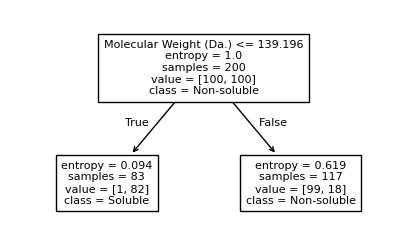
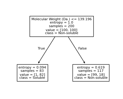
Perform decision tree classification on this dataset, let’s do the first split

[8]:
from sklearn.tree import DecisionTreeClassifier, plot_tree
from sklearn.inspection import DecisionBoundaryDisplay
[9]:
clf = DecisionTreeClassifier(random_state=42,max_leaf_nodes=2,criterion='entropy')
clf.fit(X, y)
[9]:
DecisionTreeClassifier(criterion='entropy', max_leaf_nodes=2, random_state=42)In a Jupyter environment, please rerun this cell to show the HTML representation or trust the notebook.
On GitHub, the HTML representation is unable to render, please try loading this page with nbviewer.org.
DecisionTreeClassifier(criterion='entropy', max_leaf_nodes=2, random_state=42)
[10]:
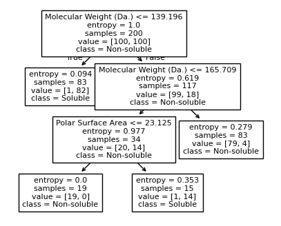
plt.figure(figsize=(5, 3))
plot_tree(clf, filled=False, feature_names=["Molecular Weight (Da.)", "Polar Surface Area"], class_names=["Non-soluble", "Soluble"], fontsize=8)
[10]:
[Text(0.5, 0.75, 'Molecular Weight (Da.) <= 139.196\nentropy = 1.0\nsamples = 200\nvalue = [100, 100]\nclass = Non-soluble'),
 Text(0.25, 0.25, 'entropy = 0.094\nsamples = 83\nvalue = [1, 82]\nclass = Soluble'),
 Text(0.375, 0.5, 'True  '),
 Text(0.75, 0.25, 'entropy = 0.619\nsamples = 117\nvalue = [99, 18]\nclass = Non-soluble'),
 Text(0.625, 0.5, '  False')]
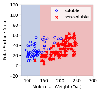
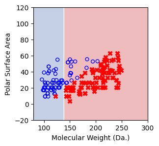
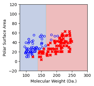
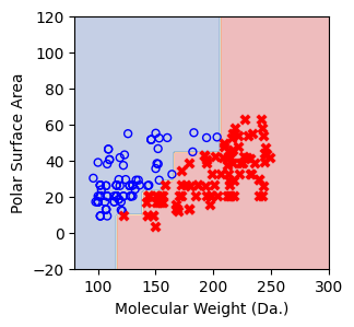
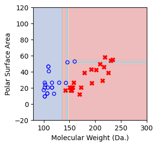
Visualize the predicted regions from one-split decision tree model.
In this visualization, the blue region indicates that the model predicts the points within this area as soluble and vice versa
[11]:
a = np.arange(80,301,0.1)
b = np.arange(-20,121,0.1)
aa,bb = np.meshgrid(a,b)
X_grid = np.concatenate([aa.ravel().reshape(-1,1),bb.ravel().reshape(-1,1)],axis=1)

f, ax = plt.subplots(1,1,figsize=(3,3))
#plt.tight_layout(h_pad=0.5, w_pad=0.5, pad=2.5)
DecisionBoundaryDisplay.from_estimator(
    clf,
    X_grid,
    cmap=plt.cm.RdYlBu,
    response_method="predict",
    ax=ax,
    alpha=0.3,
)
ax.scatter(X[np.where(y==1)[0],0],X[np.where(y==1)[0],1],s=25, marker='o', facecolors='none', edgecolor="blue", label='soluble')
ax.scatter(X[np.where(y==-1)[0],0],X[np.where(y==-1)[0],1],s=50, marker='X', color='red',linewidths=0.1, label='non-soluble')

ax.set_xlabel("Molecular Weight (Da.)")
ax.set_ylabel("Polar Surface Area")

ax.set_xlim(80,300)
ax.set_ylim(-20,120)

plt.legend()
[11]:
<matplotlib.legend.Legend at 0x7e57e154f6e0>
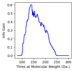
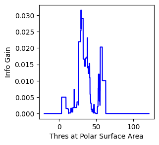
You can manually write the info gain formula to find the split, which is consistent with result from sklearn

[12]:
def entropy(p):
    return -p*np.log2(p) - (1-p)*np.log2(1-p)

def infogain(X,y,thres,axis=0):

    pos = len(np.where(y==1)[0])
    neg = len(np.where(y==-1)[0])

    if pos == 0 or neg == 0:
        Hy = 0
    else:
        Hy = entropy(pos/(pos+neg))

    idx0 = np.where(X[:,axis]<=thres)[0]
    idx1 = np.where(X[:,axis]>thres)[0]

    p0 = len(idx0)/(len(idx0)+len(idx1))
    p1 = 1 - p0

    y0 = y[idx0]
    pos = len(np.where(y0==1)[0])
    neg = len(np.where(y0==-1)[0])
    if pos == 0 or neg == 0:
        Hy0 = 0
    else:
        Hy0 = entropy(pos/(pos+neg))

    y1 = y[idx1]
    pos = len(np.where(y1==1)[0])
    neg = len(np.where(y1==-1)[0])
    if pos == 0 or neg == 0:
        Hy1 = 0
    else:
        Hy1 = entropy(pos/(pos+neg))

    HySplit = p0*Hy0 + p1*Hy1

    return Hy-HySplit
[13]:
# scan the first feature of molecular weight
thres = np.arange(80,301,0.1)
ig = []
for i in thres:
    ig.append(infogain(X,y,i,axis=0))

f, ax = plt.subplots(1,1,figsize=(3,3))
ax.plot(thres,ig,c='blue')

ax.set_xlabel("Thres at Molecular Weight (Da.)")
ax.set_ylabel("Info Gain")
[13]:
Text(0, 0.5, 'Info Gain')
[14]:
# scan the second feature of polar surface area
thres = np.arange(-20,121,0.1)
ig = []
for i in thres:
    ig.append(infogain(X,y,i,axis=1))

f, ax = plt.subplots(1,1,figsize=(3,3))
ax.plot(thres,ig,c='blue')

ax.set_xlabel("Thres at Polar Surface Area")
ax.set_ylabel("Info Gain")
[14]:
Text(0, 0.5, 'Info Gain')
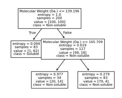
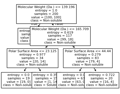
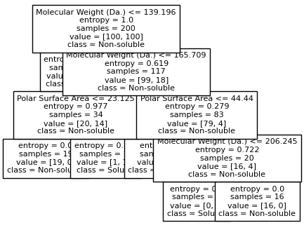
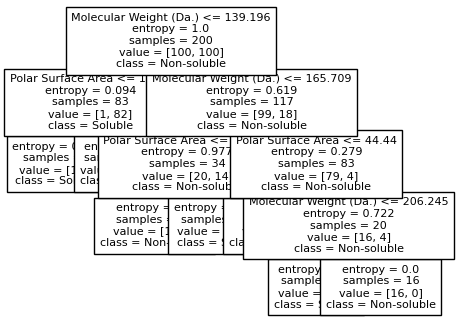
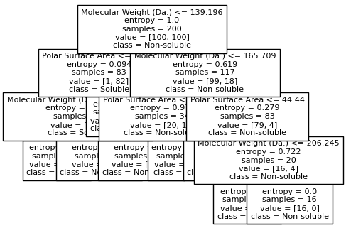
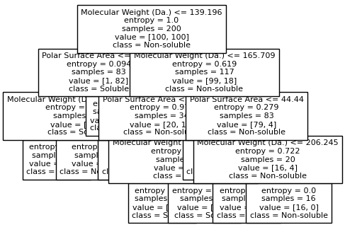
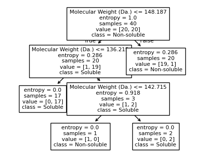
Split until all data points are correctly classified
[15]:
for num_nodes in range(2,20):

    clf = DecisionTreeClassifier(random_state=42,max_leaf_nodes=num_nodes,criterion='entropy')
    clf.fit(X, y)
    # when score == 1, indicating that all data points are correctly classified
    score = clf.score(X, y)

    plt.figure(figsize=(5, 4))
    plot_tree(clf, filled=False, feature_names=["Molecular Weight (Da.)", "Polar Surface Area"], class_names=["Non-soluble", "Soluble"], fontsize=8)


    a = np.arange(80,301,0.1)
    b = np.arange(-20,121,0.1)
    aa,bb = np.meshgrid(a,b)
    X_grid = np.concatenate([aa.ravel().reshape(-1,1),bb.ravel().reshape(-1,1)],axis=1)

    f, ax = plt.subplots(1,1,figsize=(3,3))
    #plt.tight_layout(h_pad=0.5, w_pad=0.5, pad=2.5)
    DecisionBoundaryDisplay.from_estimator(
        clf,
        X_grid,
        cmap=plt.cm.RdYlBu,
        response_method="predict",
        ax=ax,
        alpha=0.3,
    )
    ax.scatter(X[np.where(y==1)[0],0],X[np.where(y==1)[0],1],s=25, marker='o', facecolors='none', edgecolor="blue", label='soluble')
    ax.scatter(X[np.where(y==-1)[0],0],X[np.where(y==-1)[0],1],s=50, marker='X', color='red',linewidths=0.1, label='non-soluble')

    ax.set_xlabel("Molecular Weight (Da.)")
    ax.set_ylabel("Polar Surface Area")

    ax.set_xlim(80,300)
    ax.set_ylim(-20,120)

    if score == 1.:
        break


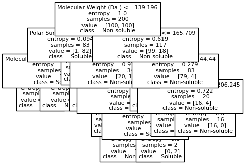
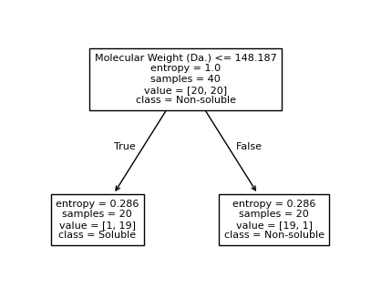
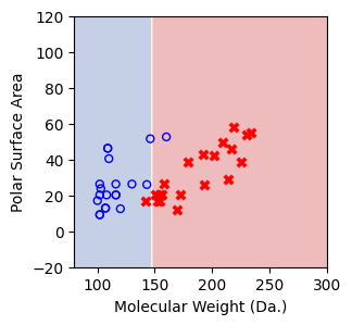
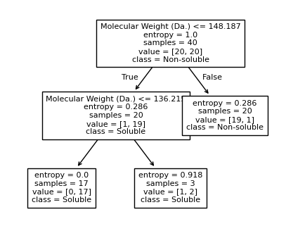
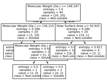
We then show decision tree is not robust to noisy data, lets use 40 compounds dataset again
[16]:
df = pd.read_csv('delaney_dataset_40compounds.csv')
df.head(2)

data = df.iloc[:].values

# data with Molecular Weight and Polar Surface Are as features.
X = data[:,0:2]

# solubility labels
y = data[:,3].astype(int)
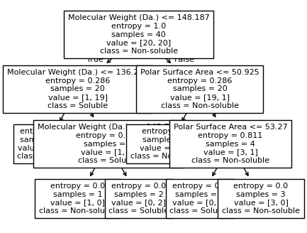
[17]:
for num_nodes in range(2,20):

    clf = DecisionTreeClassifier(random_state=42,max_leaf_nodes=num_nodes,criterion='entropy')
    clf.fit(X, y)
    # when score == 1, indicating that all data points are correctly classified
    score = clf.score(X, y)

    plt.figure(figsize=(5, 4))
    plot_tree(clf, filled=False, feature_names=["Molecular Weight (Da.)", "Polar Surface Area"], class_names=["Non-soluble", "Soluble"], fontsize=8)


    a = np.arange(80,301,0.1)
    b = np.arange(-20,121,0.1)
    aa,bb = np.meshgrid(a,b)
    X_grid = np.concatenate([aa.ravel().reshape(-1,1),bb.ravel().reshape(-1,1)],axis=1)

    f, ax = plt.subplots(1,1,figsize=(3,3))
    #plt.tight_layout(h_pad=0.5, w_pad=0.5, pad=2.5)
    DecisionBoundaryDisplay.from_estimator(
        clf,
        X_grid,
        cmap=plt.cm.RdYlBu,
        response_method="predict",
        ax=ax,
        alpha=0.3,
    )
    ax.scatter(X[np.where(y==1)[0],0],X[np.where(y==1)[0],1],s=25, marker='o', facecolors='none', edgecolor="blue", label='soluble')
    ax.scatter(X[np.where(y==-1)[0],0],X[np.where(y==-1)[0],1],s=50, marker='X', color='red',linewidths=0.1, label='non-soluble')

    ax.set_xlabel("Molecular Weight (Da.)")
    ax.set_ylabel("Polar Surface Area")

    ax.set_xlim(80,300)
    ax.set_ylim(-20,120)

    if score == 1.:
        break


[17]: