CHEM361 - Reference Jupyter Notebook for Homework 1
This notebook demonstrates
How to use
rdkitto load molecules, calculate molecular properties, calculate morgan fingerprints.How to use clustering and dimensionality reduction methods available in
scikit-learn(akasklearn) on chemical compounds to discover underlying patterns.
1. Install Dependencies and Download Dataset
The packages and dataset required in this assignment are the same as in “homework0_reference.ipynb”.
[ ]:
!pip install pandas matplotlib rdkit scikit-learn wget

!python -m wget https://raw.githubusercontent.com/deepchem/deepchem/master/datasets/delaney-processed.csv \
    --output delaney-processed.csv
2. Molecular Representations
2.1 Load Molecule from SMILES
We will practice about how to load molecule from SMILES in RDKit.
rdkit can convert any valid SMILES to a molecule automatically. Firstly, we import rdkit.Chem module that contains basic functions for woriking with small molecules, such as loading molecules and calculating molecular properties.
[2]:
import rdkit.Chem as Chem
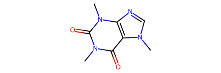
# caffeine
smi = "Cn1c(=O)c2c(ncn2C)n(C)c1=O"
mol = Chem.MolFromSmiles(smi)
mol
[2]:

2.2 Canonical SMILES
Convert the molecule to canonical SMILES
[3]:
Chem.MolToSmiles(mol, canonical=True)
[3]:
'Cn1c(=O)c2c(ncn2C)n(C)c1=O'
Similarly, you can try the other two SMILES examples for caffeine mentioned in the lecture.
Below is the SMILES string for Caffeine from PubChem
CN1C=NC2=C1C(=O)N(C(=O)N2C)C

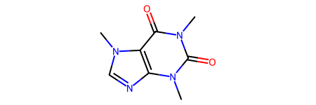
[4]:
smi1 = "CN1C=NC2=C1C(=O)N(C(=O)N2C)C"
mol1 = Chem.MolFromSmiles(smi1)
can_smi1 = Chem.MolToSmiles(mol1, canonical=True)
print(f"The canonical SMILES in RDKit for {smi1} is {can_smi1}")
mol1
The canonical SMILES in RDKit for CN1C=NC2=C1C(=O)N(C(=O)N2C)C is Cn1c(=O)c2c(ncn2C)n(C)c1=O
[4]:
Below is another SMILES string for Caffeine:
CN1C(=O)C2=C(N=CN2C)N(C)C1=O

[5]:
smi2 = "CN1C(=O)C2=C(N=CN2C)N(C)C1=O"
mol2 = Chem.MolFromSmiles(smi2)
can_smi2 = Chem.MolToSmiles(mol2, canonical=True)
print(f"The canonical SMILES in RDKit for {smi2} is {can_smi2}")
mol2
The canonical SMILES in RDKit for CN1C(=O)C2=C(N=CN2C)N(C)C1=O is Cn1c(=O)c2c(ncn2C)n(C)c1=O
[5]:
The above results show that three SMILES strings for caffeine discussed in the lecture. However, according to the canonical SMILES string scheme in RDkit, the following one:"Cn1c(=O)c2c(ncn2C)n(C)c1=O" is canonical.
However, if you look up the caffeine CID2519 in the PubChem database, you’ll notice that PubChem uses a different canonical SMILES string "CN1C=NC2=C1C(=O)N(C(=O)N2C)C". This difference arises because there are multiple canonicalization algorithms.
Note: Don’t worry too much about canonical SMILES if your primal goal is to use SMILES for loading molecules. However, if you need a one-to-one mapping between a molecule and its SMILES, make sure to stick to one specific canonicalization algorithm.
2.3. Morgan Fingerprints and Bit Collisions
RDKit.Chem.AllChem contains more advanced functions, such as calculating fingerprints and generating molecular conformation. To calculate Morgan fingerprint, we need to pass in a radius parameter radius and a length parameter nBits.
Don’t worry if you see a deprecation warning when using AllChem.GetMorganFingerprintAsBitVect function, this function still works.
[6]:
import rdkit.Chem.AllChem as AllChem

fp = AllChem.GetMorganFingerprintAsBitVect(mol, radius=2, nBits=1024)
[16:02:35] DEPRECATION WARNING: please use MorganGenerator
[7]:
print("Positions of 1-bit:")
for idx in fp.GetOnBits():
    print(idx, end=", ")
Positions of 1-bit:
0, 33, 121, 179, 234, 283, 314, 330, 356, 378, 385, 400, 416, 428, 463, 493, 504, 564, 650, 672, 771, 849, 932, 935,
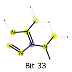
We can draw the subgraphs for the “1” bits. Firstly, we need to import the module rdkit.Chem.Draw for RDKit plotting. Secondly, we need to pass a dictionary bi to the fingerprint calculation, for storing the subgraphs.
[8]:
import rdkit.Chem.Draw as Draw

bi = {} # bit info
fp = AllChem.GetMorganFingerprintAsBitVect(mol, radius=2, nBits=2048, bitInfo=bi)

idx = 33
on_bits = [(mol, idx, bi)]
labels = [f"Bit {str(idx)}"]
Draw.DrawMorganBits(on_bits, molsPerRow=1, legends=labels)
[16:02:35] DEPRECATION WARNING: please use MorganGenerator
[8]:
2.4. Molecular Properties
The rdkit.Chem.Descriptors module contains a wide variety of molecular descriptors that can be directly accessed to compute additional properties for molecules. For example, we can calculate some basic molecular descriptors:
[9]:
import numpy as np
import rdkit.Chem.Descriptors as Descriptors
property_array = np.array([
    Descriptors.MolWt(mol),
    Chem.Lipinski.NumHAcceptors(mol),
    Chem.Lipinski.NumHDonors(mol),
    Chem.Lipinski.RingCount(mol)
])
print("Custom molecular descriptor array:", property_array)
Custom molecular descriptor array: [194.194 6. 0. 2. ]
The concept of “drug-likeness” often involves applying specific rules or scoring functions, such as Lipinski’s Rule of Five or the QED (Quantitative Estimation of Drug-likeness) as described in the paper “Quantifying the chemical beauty of drugs” (Nature Chemistry, 2012).
RDKit implements QED directly, making it easy to compute drug-likeness scores for molecules.
[10]:
# quantitative estimation of drug-likeness (QED)
q = Descriptors.qed(mol)
print("QED of caffeine:", q)
QED of caffeine: 0.5384628262372215
More scripts and workflows developed by the community are available at the rdkit.Contrib. The is not a module that can be imported directly. If you want to calculate the synthetic accessibility score (SAScore) of molecules in organic synthesis, you can use the following blocks to:
download scripts from the repository
add the script to the system path
import thhe script and do calculation
[11]:
## Download source code to compute synthetic availability score from rdkit
!python -m wget https://raw.githubusercontent.com/rdkit/rdkit/master/Contrib/SA_Score/sascorer.py
!python -m wget https://raw.githubusercontent.com/rdkit/rdkit/master/Contrib/SA_Score/fpscores.pkl.gz
Saved under sascorer.py

Saved under fpscores.pkl.gz
[12]:
import os, sys
from rdkit.Chem import RDConfig
# using literature contributors
# from https://github.com/rdkit/rdkit/tree/master/Contrib
sys.path.append(os.path.join(RDConfig.RDContribDir, 'SA_Score'))

import sascorer
s = sascorer.calculateScore(mol)
print("Synthetic Availability:", s)
Synthetic Availability: 2.29798245679401
3. Work on a Dataset
You are an expert in SMILES, molecular properties, and fingerprints. In this section, we will explore how to apply the functions mentioned in the above section to multiple molecules.
3.1 Load Dataset
[13]:
import pandas as pd

DELANEY_FILE = "delaney-processed.csv"
df = pd.read_csv(DELANEY_FILE)
print(f"Number of molecules in the dataset: {df.shape[0]}")
Number of molecules in the dataset: 1128
[14]:
df.head(5)
[14]:
| Compound ID | ESOL predicted log solubility in mols per litre | Minimum Degree | Molecular Weight | Number of H-Bond Donors | Number of Rings | Number of Rotatable Bonds | Polar Surface Area | measured log solubility in mols per litre | smiles | |
|---|---|---|---|---|---|---|---|---|---|---|
| 0 | Amigdalin | -0.974 | 1 | 457.432 | 7 | 3 | 7 | 202.32 | -0.77 | OCC3OC(OCC2OC(OC(C#N)c1ccccc1)C(O)C(O)C2O)C(O)... |
| 1 | Fenfuram | -2.885 | 1 | 201.225 | 1 | 2 | 2 | 42.24 | -3.30 | Cc1occc1C(=O)Nc2ccccc2 |
| 2 | citral | -2.579 | 1 | 152.237 | 0 | 0 | 4 | 17.07 | -2.06 | CC(C)=CCCC(C)=CC(=O) |
| 3 | Picene | -6.618 | 2 | 278.354 | 0 | 5 | 0 | 0.00 | -7.87 | c1ccc2c(c1)ccc3c2ccc4c5ccccc5ccc43 |
| 4 | Thiophene | -2.232 | 2 | 84.143 | 0 | 1 | 0 | 0.00 | -1.33 | c1ccsc1 |
3.2. Pandas DataFrame Operations
Recap in Homework 0, we created a molecule from each SMILES and stored the created molecules in a new column “mol” using the following command:
from rdkit.Chem import PandasTools
PandasTools.AddMoleculeColumnToFrame(df, "smiles", "mol")
Equivalent, we can use Chem.MolFromSmiles to create molecules:
# fetch the smiles column in df
smis = df["smiles"]

# apply Chem.MolFromSmiles for each SMILES string
# mols is a column of molecules
mols = smis.apply(lambda x: Chem.MolFromSmiles(x))

# add mols to df
df["mol"] = mols
[15]:
# get molecules from smiles
df["mol"] = df["smiles"].apply(lambda x: Chem.MolFromSmiles(x))
Morgan fingerpring of each molecule in the dataset can be calculated using df.apply together with the lambda function. Just in case the deprecated warning of AllChem.GetMorganFingerprintAsBitVect occur repeatedly, we can use a new function when calculating the fingerprints of multiple molecules.
[16]:
# rdFingerprintGenerator is recommended in the newer versions of rdkit to replace AllChem.GetMorganFingerprintAsBitVect
from rdkit.Chem import rdFingerprintGenerator

morgan_fp_gen = rdFingerprintGenerator.GetMorganGenerator(includeChirality=True, radius=2, fpSize=1024)

# morgan_fp_gen.GetFingerprint(mol) converts a mol to a fingerprint
# we use apply to convert all mols to fingerprints
df["fp"] = df["mol"].apply(lambda x: morgan_fp_gen.GetFingerprint(x))
Now let’s check the dataframe. There should be two additional columns: “mol” and “fp”.
[17]:
df.head(3)
[17]:
| Compound ID | ESOL predicted log solubility in mols per litre | Minimum Degree | Molecular Weight | Number of H-Bond Donors | Number of Rings | Number of Rotatable Bonds | Polar Surface Area | measured log solubility in mols per litre | smiles | mol | fp | |
|---|---|---|---|---|---|---|---|---|---|---|---|---|
| 0 | Amigdalin | -0.974 | 1 | 457.432 | 7 | 3 | 7 | 202.32 | -0.77 | OCC3OC(OCC2OC(OC(C#N)c1ccccc1)C(O)C(O)C2O)C(O)... | <rdkit.Chem.rdchem.Mol object at 0x00000228672... | [0, 1, 0, 0, 1, 0, 0, 0, 0, 0, 0, 0, 0, 1, 0, ... |
| 1 | Fenfuram | -2.885 | 1 | 201.225 | 1 | 2 | 2 | 42.24 | -3.30 | Cc1occc1C(=O)Nc2ccccc2 | <rdkit.Chem.rdchem.Mol object at 0x00000228672... | [0, 0, 0, 0, 0, 0, 0, 0, 0, 0, 0, 0, 0, 0, 0, ... |
| 2 | citral | -2.579 | 1 | 152.237 | 0 | 0 | 4 | 17.07 | -2.06 | CC(C)=CCCC(C)=CC(=O) | <rdkit.Chem.rdchem.Mol object at 0x00000228672... | [0, 0, 0, 0, 0, 0, 0, 0, 0, 0, 0, 0, 0, 0, 0, ... |
4. Clustering
We want to clustering using “Molecular Weight”, “Number of H-Bond Donors”, “Number of Rings” and “Number of Rotatable Bonds”. We can select these columns from the dataframe.
[18]:
# select multi-columns
X = df[["Molecular Weight", "Number of H-Bond Donors", "Number of Rings", "Number of Rotatable Bonds"]]

# keep values only, discard the df.index
X = X.values

# print the shape
print("Shape of X:", X.shape)
Shape of X: (1128, 4)
You can print the values in X to check.
[19]:
print(X)
[[457.432   7.      3.      7.   ]
 [201.225   1.      2.      2.   ]
 [152.237   0.      0.      4.   ]
 ...
 [246.359   0.      0.      7.   ]
 [ 72.151   0.      0.      1.   ]
 [365.964   0.      1.      5.   ]]
The matrix shape means that it has 1128 rows (the number of molecules), and 4 columns (the number of features we chose).
4.1 Data Normalization
As we highlighted in the lecture, data normalization is important, especially for techniques like clustering and PCA. One common way to normalize data is by using StandardScalar from the sklearn.preprocessing module. The formula for normalization is:
This scaling method substracts the mean \(\mu\) from the original data and divides by the standard deviation (\(\sigma\)), ensuring that each feature has a mean of 0 and a standard deviation of 1.
[20]:
from sklearn.preprocessing import StandardScaler

# create a scaler object
scaler = StandardScaler()

# transform X to Z, Z has a mean of 0 and std of 1
Z = scaler.fit_transform(X)
[21]:
Z
[21]:
array([[ 2.46848464,  5.78268892,  1.22109812,  1.82691435],
       [-0.02640966,  0.27428095,  0.46220077, -0.06716597],
       [-0.50344534, -0.64378704, -1.05559391,  0.69046616],
       ...,
       [ 0.41309652, -0.64378704, -1.05559391,  1.82691435],
       [-1.28330735, -0.64378704, -1.05559391, -0.44598203],
       [ 1.57778691, -0.64378704, -0.29669657,  1.06928222]],
      shape=(1128, 4))
You can calculate the mean and std of each feature using the following commands to check that StandardScalar did a good job in normalizing the data.
print("Check the mean of each feature:", Z.mean(axis=0))
print("Check the std of each feature:", Z.sdt(axis=0))
4.2 K-means Clustering
We don’t have reinvent the wheel every time we use a well-established method. After understanding the fundamentals of KMeans algorithm, we can confidently use KMeans from sklearn. There are two major decisions to make when using KMeans:
the number of clusters (
n_clusters)the initial centers
By default, sklearn.cluster.KMeans use the “k-means++” method to find initial centers. This method aims to find initial centers that are spread out, which helps improve the performance and convergence of the algorithm.
[22]:
from sklearn.cluster import KMeans

# please explore n_clusters
n_clusters = 3

k_means = KMeans(n_clusters, init="k-means++")

# fit data
k_means.fit(Z)

# fetch predicted labels for each datapoint
labels = k_means.labels_
c:\Users\24153\anaconda3\envs\chem361\lib\site-packages\sklearn\cluster\_kmeans.py:1411: UserWarning: KMeans is known to have a memory leak on Windows with MKL, when there are less chunks than available threads. You can avoid it by setting the environment variable OMP_NUM_THREADS=5.
  warnings.warn(
We can find the number of molecules in each cluster (cluster size).
[23]:
# you can use for-loop to find out the size, but here's a quicker way
from collections import Counter
Counter(labels)
[23]:
Counter({np.int32(0): 647, np.int32(2): 324, np.int32(1): 157})
Let’s fetch the value of loss function (sum of squared distance)
[24]:
ssd = k_means.inertia_
print(f"Sum of squared distance after model fitting: {ssd:.2f}")
Sum of squared distance after model fitting: 2516.39
You can apply the expirical “elbo” method to pick a better n_clusters from this plot.
4.3 DBSCAN Clustering
There are two major decisions to make when using DBSCAN:
the distance
epsused to build \(\epsilon\)-neighbourhoodthe minimum number of neighbours
min_samplesto determine core points
It is important to note that
[25]:
from sklearn.cluster import DBSCAN

eps = 0.5
min_samples = 5

dbscan = DBSCAN(eps=eps, min_samples=min_samples, \
    metric="euclidean", algorithm="auto")

dbscan.fit(Z)
[25]:
DBSCAN()In a Jupyter environment, please rerun this cell to show the HTML representation or trust the notebook.
On GitHub, the HTML representation is unable to render, please try loading this page with nbviewer.org.
DBSCAN()
You can find out the number of clusters after DBSCAN clustering, but pay attention to points with cluster label as -1. These points are noise, not clustered.
[26]:
counter = Counter(dbscan.labels_)
# remove cluster_id=-1
counter.pop(-1)

print("Number of clusters:", len(counter))
print("Size of each cluster:", counter)
Number of clusters: 18
Size of each cluster: Counter({np.int64(1): 223, np.int64(3): 150, np.int64(5): 118, np.int64(4): 107, np.int64(10): 62, np.int64(7): 60, np.int64(0): 53, np.int64(11): 42, np.int64(6): 35, np.int64(8): 30, np.int64(9): 28, np.int64(12): 24, np.int64(15): 16, np.int64(13): 10, np.int64(2): 9, np.int64(16): 7, np.int64(14): 5, np.int64(17): 5})
5. Dimensionality Reduction using PCA
5.1 PCA on Molecular Descriptors
PCA should also use data after remove mean. Therefore, we still use \(Z\) matrix.
[27]:
from sklearn.decomposition import PCA
n_components = 1
pca = PCA(n_components=n_components)
pca.fit(Z)

Z_reduced = pca.transform(Z)
print("Shape of the reduced matrix:", Z_reduced.shape)
Shape of the reduced matrix: (1128, 1)
The we fetch the vectors of pricipal components (the eigenvectors we mentioned in lecture).
[28]:
# principal components
pca.components_
[28]:
array([[0.67953142, 0.37265949, 0.5759563 , 0.2600698 ]])
I need to emphasize on the shape of input Z, the output Z_reduced and the PCs pca.components_. Z has the shape of (1128, 4), Z_reduced has the shape of (1128, 1), and pca.components_ has the shape of \((1, 4)\). The input and output of sklearn.decomposition.PCA are on the row space, while in equations in lecture are on the column space. Both are correct.